A Survey of Light Estimation Analysis
For my final project in CS 283 (Computer Vision) I decided to examine strategies for reconstructing the lighting conditions of a scene given an image, for the ultimate purpose of properly lighting AR objects in a “magic mirror” device. The write up is republished below, with a few changes to make the results clearer at a glance. Enjoy!
Author: Nicolas Chavez
Course: Harvard CS 283
Instructor: Professor Todd Zickler
I. Introduction
Light estimation analysis has been studied since 1975 by S. Ullman [1], who worked with a very simple case – estimating light sources that were visible in the image. Since then, substantial progress has been made in the field, using very different methods, such as using light probes, multiple shots of a scene, or lighting assumptions. The methods developed are of varying use depending on the situation or application.
Common applications include scene reconstruction, augmented reality and photo editing.
Scene reconstruction requires point matching in a scene, which is usually easily done when objects have many features points for an algorithm like SIFT to track. However, when an objects lacks textures that do this, resolving the geometric shape from the shading of the object can lead to better tracking of points across images.
Augmented reality and photo editing both deal with inserting virtual and/or other images into video or photo. To do so realistically, these systems must present this inserted object with lighting consistent with the rest of the scene. Rendering this object with the lighting information of the scene – this includes shading, illumination, and shadows – results in very convincing overlays for users of augmented reality.
The motivation for this survey is for the application geared more toward augmented reality. More specifically, I aim to build a system called a “Magic Mirror”, which is essentially a semi-reflective surface that can have a display behind it. With a camera mounted to the the mirror, the display can overlay objects onto the user’s reflection, such as clothing or health information. To perform these processes realistically, the lighting information of the scene must be known. The scope of this is then slightly more specific since the focus is on finding the lighting information where the scene will probably contain a human in it.
The goal of this project is to survey 2 different methods to reconstruct this information and to analyze which one is more accurate given the scenario they will be applied to. In particular, there may only be a few lighting sources, and it may even be possible to approximate the lighting with one source.
II. Methods
The two methods to be analyzed are what I call “Method A”, which is developed by Moreno et. al [2], and “Method B”, which is developed by Bouganis et. al [3]. I describe both subsequently:
“Method A” calculates the number of lights in the scene, their spherical coordinates, and their relative intensities. “Method A” assumes that lighting is directional in nature and can calculate any number of lights. “Method A”, however, requires as input, the specification of the outline or silhouette of an object in the image. This object must be fully contained in the image and must contain no cavities. With this information alone, “Method A” can perform.
“Method B” calculates the number of lights in the scene, their spherical coordinates and their relative intensities as well. “Method B” also assumes that the lighting in the scene is directional, but can only calculate up to 3 light sources. Unlike “Method A”, “Method B” doesn’t require any information specific to the scene, such as a makeshift light probe, which is “Method A”’s strategy. Instead, since “Method B” relies on knowing that its input will be human faces, it requires a database of training data. This can be extended to any “class” of images, so long as they do not have cavities and are fully contained within the image.
A more in depth analysis of both methods follows:
Once “Method A” is provided with the outline/silhouette data (which is usually a binary mask over the object), it starts an iterative method to detect the number of lights in the scene and their angle in the image plane. It does this by scanning along the pixels on the edge of the object specified – the brightest parts indicate a light in that direction or a combination of lights’ effects there. Using a modified k-means grouping, it groups the different pixels into groups, where each “group” represents the light source that most explains the intensity of the pixel. However, it is clear that a point on the object is not influenced by just one light source, but potentially (most likely) a combination of them. Thus, it is a weighted k-means, where the pixel grouping is weighted to the lights in the way they affect them. This process is done iteratively until the angles of the lights converge to stable values.
After the number of lights are calculated, as well as their image-plane angles (also called the azimuth), the angle out of the image and their relative intensities are calculated. To do so, for each light source, the algorithm scans across the interior of the object along all lines parallel to the image-plane angle of the light source, calculated in the last step. Along these scans, the first local maxima/minima is selected and used to calculate the angle outside of the image plane (zenith angle). This is done after the image has undergone a bilateral filter, which removes high frequency information usually derived from texture, which interferes with the lower frequency shading information we are interested in. Once the position along the scan line is found, we calculate the normal by assuming an elliptical shape coming out of the image plane along the scan line. Doing this produces a normal, whose angle is used as the zenith angle.
Once these zenith angles are calculated, the relative intensities of the lights are calculated by weighing the pixel intensities by the now known light sources – the surface normal are assumed, the lighting parameters are known and so are the resultant intensities. With this we are able to calculate the relative intensities of each light by weighing each intensity appropriately.
“Method B” operates in the following way:
The training set is preprocessed for use later – the data comes in the following format: each image is the face of an individual’s face under 1 to 3 direction lights. Each image is also tagged with information on the direction, quantity, and intensity of these lights. With the database, the algorithm forms a generic 3D model of the “class of object”, in this case, the human face, from which it works with moving forward. Before this, however, all variation in the images not related to the lighting, such as differences in expression, albedo and facial structure are minimized in order to deliver the “generic 3D model” against which all other query face images will be transformed similarly.
This model is chosen using someone’s face that minimizes the variation in brightness across images of the same lighting. Afterwards, very variable features such as eyes, nostrils and ends of the mouth are removed from the image analysis.
Once this preprocessing is done, the algorithm is ready to analyze a given image. The basic strategy is to find the linear combination of lighting conditions that produce the given image. Using probabilistic techniques, a random vector that represents this linear combination is applied to the “generic 3D model face” and it is tested how well this matches the given image. Then, in an iterative fashion, a stochastic gradient descent is performed to find the minimum error. The seed for the stochastic gradient descent is chosen randomly, and the entire process can be done a number of times for more accurate results. The authors describe other, very similar methods that use some decomposition before hand to determine what other areas should be removed to reduce facial variability.
For my evaluation of both methods, I implemented them myself, using the same YALE face database [4] referenced by Bouganis et. al. For “Method A”, which requires the outline of an object to be indicated, I supplied a binary mask I created using Adobe Photoshop’s magic wand and quick selection tools.
To be able to test my results, I collected natural images where the light sources were known as well as synthetic images I generated using Blender, a 3D model creation and manipulation tool. Lastly, I also collected and created natural and synthetic images of human faces. These results follow.
III. Results
Synthetic Image 1
Method A
| Measure | Actual | Predicted | Error |
|---|---|---|---|
| Azimuth 1 | 310.00d | 315.04d | +5.04d |
| Azimuth 2 | 240.00d | 242.14d | +2.14d |
| Azimuth 3 | 270.00d | 272.47d | +2.47d |
| Zenith 1 | 25.00d | 25.92d | +0.92d |
| Zenith 2 | 10.00d | 10.93d | +0.93d |
| Zenith 3 | 70.00d | 69.60d | -0.40d |
| Intensity 1 | 1.00 | 1.00 | +0.00 |
| Intensity 2 | 0.50 | 0.54 | +0.04 |
| Intensity 3 | 0.25 | 0.32 | +0.07 |
Synthetic Image 2
Method A
| Measure | Actual | Predicted | Error |
|---|---|---|---|
| Azimuth 1 | 60.00d | 61.98d | +1.98d |
| Azimuth 2 | 140.00d | 147.89d | +7.89d |
| Azimuth 3 | 270.00d | 264.47d | -5.53d |
| Zenith 1 | 65.00d | 64.41d | -0.59d |
| Zenith 2 | 50.00d | 46.30d | -3.70d |
| Zenith 3 | -40.00d | -37.65d | +2.35d |
| Intensity 1 | 0.50 | 0.54 | +0.04 |
| Intensity 2 | 1.00 | 1.00 | +0.00 |
| Intensity 3 | 0.25 | 0.35 | +0.10 |
Method B
| Measure | Actual | Predicted | Error |
|---|---|---|---|
| Azimuth 1 | 60.00d | 61.48d | +1.48d |
| Azimuth 2 | 140.00d | 139.70d | -0.30d |
| Azimuth 3 | 270.00d | 272.67d | +2.67d |
| Zenith 1 | 65.00d | 66.61d | +1.61d |
| Zenith 2 | 50.00d | 48.40d | -1.6d |
| Zenith 3 | -40.00d | -40.56d | -0.56d |
| Intensity 1 | 0.50 | 0.49 | -0.01 |
| Intensity 2 | 1.00 | 1.00 | +0.00 |
| Intensity 3 | 0.25 | 0.23 | -0.02 |
Natural Image 1
Method A
| Measure | Actual | Predicted | Error |
|---|---|---|---|
| Azimuth 1 | 63.50d | 78.31d | +14.81d |
| Azimuth 2 | 147.60d | 153.70d | +6.10d |
| Zenith 1 | 55.60d | 57.36d | +1.76d |
| Zenith 2 | 71.30d | 67.63d | -3.67d |
| Intensity 1 | 1.00 | 1.00 | +0.00 |
| Intensity 2 | 1.00 | 0.89 | -0.11 |
Natural Image 2

Method A
| Measure | Actual | Predicted | Error |
|---|---|---|---|
| Azimuth 1 | 193.20d | 221.21d | +28.01d |
| Azimuth 2 | 132.70d | 118.86d | -13.84d |
| Zenith 1 | 94.00d | 10.41d | -83.59d |
| Zenith 2 | 42.90d | 5.01d | -37.89d |
| Intensity 1 | 0.60 | 1.00 | +0.40 |
| Intensity 2 | 1.00 | 0.92 | -0.08 |
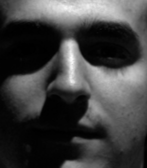
Natural Human Face 1
Method A
| Measure | Actual | Predicted | Error |
|---|---|---|---|
| Azimuth | 90.00d | 115.91d | +25.91d |
| Zenith | 20.00d | 40.65d | +20.65d |
Method B
| Measure | Actual | Predicted | Error |
|---|---|---|---|
| Azimuth | 90.00d | 88.77d | -1.23d |
| Zenith | 20.00d | 19.30d | -0.70d |
Natural Human Face 2
Method A
| Measure | Actual | Predicted | Error |
|---|---|---|---|
| Azimuth | 55.00d | 82.69d | +27.69d |
| Zenith | 65.00d | 102.11d | +57.11d |
Method B
| Measure | Actual | Predicted | Error |
|---|---|---|---|
| Azimuth | 55.00d | 40.10d | -9.90d |
| Zenith | 65.00d | 30.41d | -34.59d |
IV. Conclusion
It turns out that “Method A” is pretty accurate when analyzing the synthetic images, which is expected, since there is no noise, distortion, overly complex texture, cavities, or anything that would throw it off. It works well on the synthetic human face as well, which in this case, does not exhibit the effect of subsurface scattering a human face would have around areas of thin flesh, such as the nose or ears. Additionally, the synthetic face does not have any cast shadows or inter surface reflection at great effect.
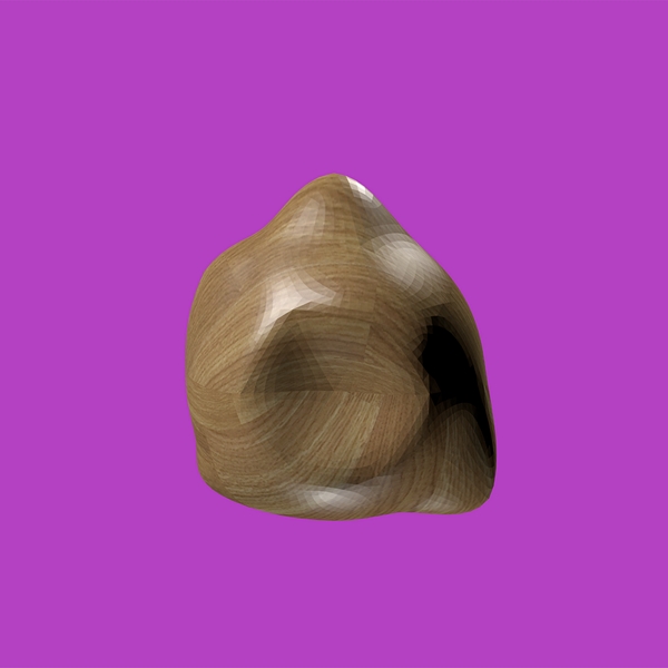
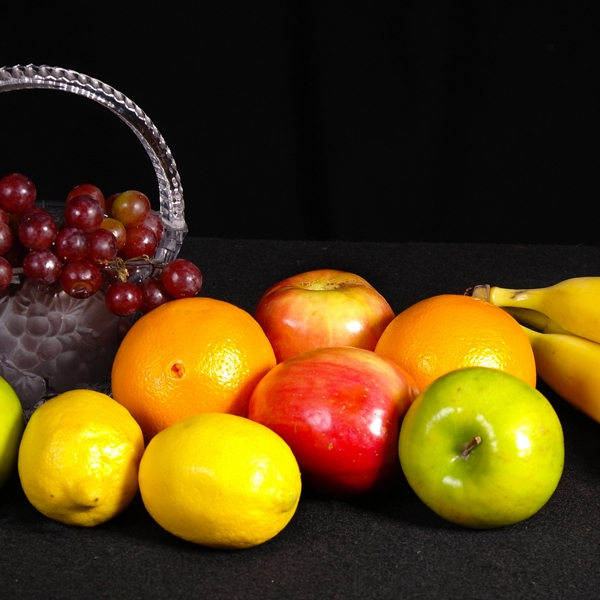
For the natural images, “Method A” does not work as well – it does a decent job for the fruit still life, in which the rightmost lemon was selected as the “makeshift probe”. This is because the lemon has a relatively Lambertian texture, with most bumps removed by the bilinear filtering. However, for the toy monkey, the furriness of the outline seems to confound the azimuth selection process, and the quick intensity variation along the interior of the object also makes the zenith selection process quit at very small angles while it searches for maxima/minima. With this, it does a poor job.
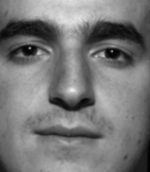
Lastly, for the natural human faces, “Method A” works fair to poorly since it was not directly possible to select an object in the image – the outline of the face was not visible. Instead, I selected the noses as the probe, since their normal does come very close to completely horizontal at the ends of the sides. It does especially poor in the second one, in which the image is dominated by cast shadows.
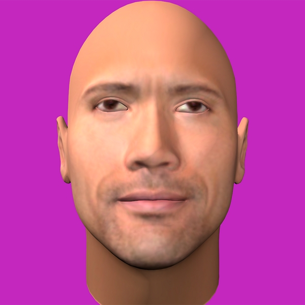
I did not bother to test “Method B” on the images that were not of human faces since it had not been optimized or trained on images not of human faces. On the synthetic face, it did a great job, which was surprising, since I expected there to be something that the 3D rendering missed that was present in real life. It is possible that the face was already very “generic” in that the albedo was very slight and not very variable (no moles, constant skin tone).
On the natural images, it performed well, slightly worse than on the synthetic image, but poorly to fair on the second, where the cast shadows were present. The optimization done during the preprocessing seems to work well for these photos, where the model was training on similar data (the natural faces were taken from the YALE database, but these in particular were excluded form the database given to the algorithm).
In conclusion, it is clear that “Method A”, or Moreno et. al’s method is more versatile in general and can work well on human faces, though it is rarely the case that applications involving human faces will be able to have users manually select a human face. In this case, it is possible to combine this method with facial recognition to recognize the outline of the face and then feed this into the algorithm. The elliptical normal assumption does not work well here in this case, and it seems like using a “generic 3D face” to base this off of would be a good idea.
“Method B”, or Bouganis et. al’s method works better than “Method A” at human faces, but can fall behind if the above optimizations are made to the first. This method could be improved if it took cast shadows into account somehow, perhaps by recognizing that on a human face these tend to happen over the eyes where the sources are “above” the face, whatever this is determined to be. Combining the stochastic gradient descent method used in “Method B” with “Method A” could also prove to be useful – we can use the results of one as the seed for the other – “Method A” could use the seed for its initial weighted k-means grouping and “Method B” could use it for its gradient descent approach.
All in all, both methods’ approaches are different enough to merit a combination that could prove to be powerful enough to deliver robust results when focusing on a particular domain of image inputs.
V. References
- S. Ullman.: On Visual Detection of Light Sources, Artificial Intelligence Memo 333, MIT 1975
- Moreno et. al: “Light source detection in photographs”. CEIG 2009, San Sebastián, September 2009
- Bouganis et. al: “Statistical multiple light source detection”. IET Comput. Vis., Vol. 1, No. 2, June 2007
- K.C. Lee and J. Ho and D. Kriegman: “Acquiring Linear Subspaces for Face Recognition under Variable Lighting”. IEEE Trans. Pattern Anal. Mach. Intelligence, 2005, pp. 684-698