Source Code on GitHub

Overview

I built an exploration simulation game, where you travel over the Earth’s seas, discovering cities across continents, islands, and coasts. For the game logic and graphics, I used C++14, Panda3D, GLSL, and Compute Shaders. For the visual assets, I used NASA’s Visible Earth satellite imagery, GEBCO’s bathymetry data, and a modded Cannon Boat from Mario Party 64.

My inspiration for this project came off the heels of my last project, which rendered terrain for a strategy game. I wanted to experiment with rendering and navigating on a sphere, instead of the usual cartesian plane. I was also inspired Sebastian Lague’s recent project, which introduced me to the above data sources. Finally, I wanted to try a lower level implementation of some of the ideas in my last project by using C++ and OpenGL instead of using an engine like Unity.

One-Time Setup Work

As inputs, the program takes in the following images based on the NASA and GEBCO data:

Albedo

This represents the color of the Earth, minus occlusions like clouds and any shading. Visible Earth provides the albedo of the Earth in various months of the years, to show how snow and ice fade in and out. I only used this data to provide land color – my calculation of water color is described later on. This is what the March capture looks like:

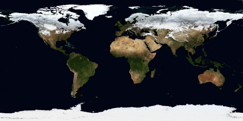
Reto Stöckli, NASA Earth Observatory, 2004.

Albedo of Earth in March. A thumbnail, since the original is a whopping 16384x8192!

Topology

This image represents the height of each land point on the Earth, where sea level is 0, and pixel intensity increases until it hits 1 at the highest point (somewhere in the Himalayas, I presume). It doesn’t capture ocean depth since water is all captured as the 0 sea level:

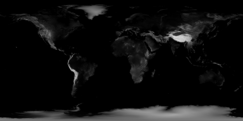
Imagery by Jesse Allen, NASA’s Earth Observatory, using data from the General Bathymetric Chart of the Oceans (GEBCO) produced by the British Oceanographic Data Centre, 2005.

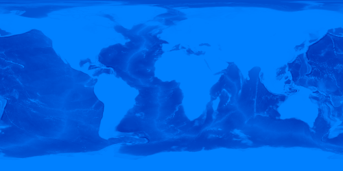
Bathymetry

This image represents the depth of each water point. At first glance, it seems to be a simple 0-1 where 0 is the deepest the ocean is (Marianas Trench, south of Japan) and then 1 for land. However, this data needed to be cleaned up a bit (using levels in GIMP) since the Marianas Trench is a bit above 0 (~0.2):

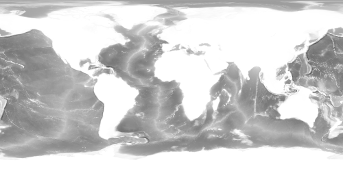
GEBCO Compilation Group (2021) GEBCO 2021 Grid (doi:10.5285/c6612cbe-50b3-0cff-e053-6c86abc09f8f)

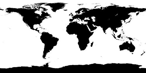
Land Mask

Finally, this image I created myself by taking the bathymetry image and thresholding it so that black pixels became land and white pixels became water. I smoothed it out a bit by using a soft threshold – instead of a hard cutoff at say 0.8, values below 0.79 became black, values above 0.81 became white, while values in between 0.79 and 0.81 were interpolated somewhere into the 0-1 range.

I also took the opportunity to remove small islands that were only a few pixels large for two reasons. For one, this image is the basis for the boat’s collision, so it would be confusing for the user if a landmass was so small, they could not see what they were colliding with. Secondly, some of these islands are so small that they don’t show up in the albedo image, instead appearing as dark ocean. As a result, they would just show up as black specks on a bright ocean (described later in this article – I color the ocean much lighter than it appears in the NASA albedo data). Via a combination of erosion and dilation kernels (i.e. opening) and manual tweaks, voilà:

Synthesis

At runtime, the program kicks off a compute shader that creates the Earth mesh, taking in the topology texture. After tessellating the sphere (a cube mesh, with all its points normalized to the unit sphere), the shader displaces the vertices according to their height by sampling the topology texture. For vertices that correspond to the water, these are left undisplaced.

In the next step, another compute shader is run to create a normal map, based on the topology and bathymetry textures. This shader simply takes the gradient of the heightmap at a given pixel and outputs that. Of course, this can be done completely offline in a tool like GIMP, or run once and saved as a predefined asset.

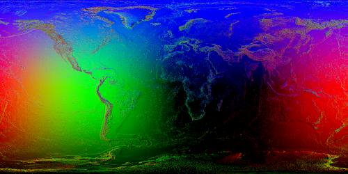
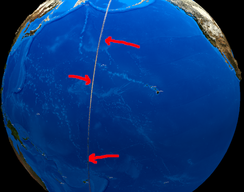
In the RHS coordinate system convention I use, +X points out of the intersection of the International Date Line and the Equator (near Hawaii), +Y points out 90 degrees to the east and at the Equator (near Colombia), and +Z points out of the North Pole. As a result, when the XYZ components of the normal vectors are encoded into RGB values (at least in the smooth parts of the globe that stay close to a spherical surface), the Pacific Ocean appears red, Latin America appears green, and the North Pole appears blue.

Of course, the noisier parts are encoding normal vectors that don’t correspond to a perfectly spherical surface, but normal vectors that correspond to rough terrain and land mass boundaries.

Per-Frame Work

The user initially starts with none of the Earth explored, but then progressively uncovers more of it as the boat travels. To make this effect, I create another texture that tracks the explored portion of the globe. In this texture, the VisibilityTex, a 0 indicates that this pixel is not yet explored, a 1 indicates that it has, and values in between are used to smooth out the effect.

On every frame, the updateVisibility compute shader is run, which takes in the boat’s current coordinates and the VisibilityTex. For pixels immediately visible by the boat (a small radius around the boat), the shader marks these as 1 (with some fading at the radius edge) and then compares this value with the existing visibility from the last frame in VisibilityTex. The max is taken and placed into VisibilityTex.

Then, when the globe is being drawn, its fragment shader samples VisibilityTex and uses it as a mask to interpolate between the Earth’s albedo for explored areas, and an empty map “incognita” texture for unexplored areas.

The empty map “terra incognita” texture

All together, the composited image after applying the visibility mask looks like this:

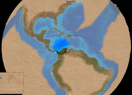
The boat is near Cartagena, Colombia. Note that the immediately visible area is the real coloring, while explored areas that are not immediately visible are duller, blended into the “terra incognita” texture a bit.

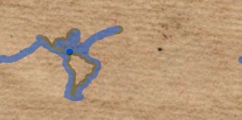
This same texture and technique is used to render the minimap, which happens to be rendered on a quad instead of a sphere (an equirectangular, or plate carrée projection!) (and with simpler textures since it’s smaller):

For determining the color for the explored portion of the Earth, as mentioned, the NASA albedo data is used for the land portions. Unfortunately, the NASA imagery leaves the oceans very dark, nearly black, which is not very exciting. Instead, the fragment shader, when drawing a water pixel, will interpolate between a light ocean color and a dark ocean color depending on bathymetry depth, which looks a lot better:

Afterwards, the data from the normal texture is used to implement diffuse lighting.

One interesting gotcha is that UV texture coordinates can’t be defined upfront when building the Earth sphere mesh at startup. This is because at the International Date Line, the texture UVs will wrap around and jump from 0.9 -> 1.0 -> 0.0 -> 0.1. This causes a visible artifact where between 1.0 and 0.0, the fragment shader interpolates the vertex UVs and renders the entire texture in a tiny sliver in reverse. To avoid this, the fragment shader instead calculates the UV based on the fragment world position. Since this happens on the fragment level and not at the vertex level, this artifact is avoided.

Whoops!

All in all, this is what the final product looks like if you’ve explored the entire planet!

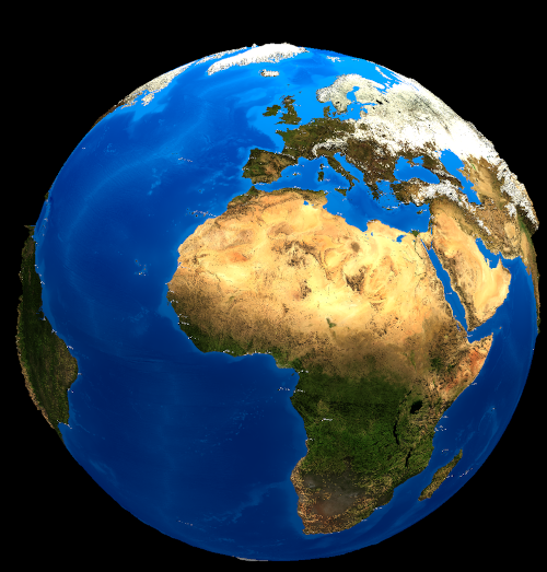
The Blue Marble :)

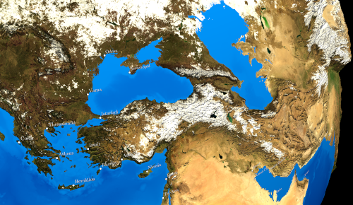
Another look at a closer angle. Notice the Himalayas coming off the sphere, on the right of the image!

Model, View, NodePath Architecture

For this project, I used the Panda3D framework to provide a scenegraph and OpenGL boilerplate. Note that Panda3D has a popular Python API, but also exposes a C++ API, which I used for this project. I had never tried Panda3D, but had read good things about it, so I decided to give it a try.

Like in my previous projects, I tried to design the program in a way that decouples the model from the view, and allowed the application to precisely determine what per-frame work needed to be done. One thing that was unintuitive in this project was that the NASA and GEBCO texture data seemed like they were firmly in the “view” domain, but in reality, since this texture data was used for determining collisions, it actually belonged in the “model” domain!

To that end, I split up the Globe class roughly as such, one for model, one for view:

// The data model, pseudocode
class Globe {
 public:
  Globe(
    // needed to run compute shaders
    GraphicsOutput *gfx_output,
    Texture *topology_tex,
    Texture *bathymetry_tex,
    Texture *land_mask_tex,
    Texture *albedo_tex,
    Texture *visibility_tex);

  bool isLandAtPoint(Point p) const;
  float getHeightAtPoint(Point p) const;
  void updateVisibility(GraphicsOutput *gfx_output, Point player_position);
};

To understand the view, one must understand how Panda3D renders an object. Generally, to render something in Panda3D, you attach a Node to another (and at the top, the scenegraph root node). This creates a NodePath, which points to this node using a path description, sort of like a URL. There are a few Node subclasses that Panda3D provides, one of which is for procedurally generated mesh data (used in this case). However, setting materials, transforms, and other attributes common to all node types are operations performed on the NodePath object. Thus, GlobeView below is rather simple, as it is just responsible for creating this initial mesh Node by invoking the compute shader, and setting the appropriate vertex and fragment shaders and textures on the NodePath.

// The view, for rendering
class GlobeView {
 public:
  GlobeView(GraphicsOutput *gfx_output, Globe &globe);

  NodePath getPath() const;
};

In hindsight, while workable, I don’t think this design pattern was a good match with Panda3D. With Unity, each XYZView was a component MonoBehaviour script, and hierarchies between views were reflected in GameObject transform hierarchies, so views and the underlying engine objects were intertwined.

In Panda3D, applying this pattern led to 3 object graphs: one for the model, one for the view, and one for the Panda3D scene. This made ownership more difficult to reason about, as destroying a NodePath didn’t necessarily destroy its corresponding view object.

Future Work

Going forward, I’d like to go even lower level and interact more directly with OpenGL (or similar), in order to have more control over what graphics work is being performed each frame. Additionally, I’m intrigued by ECS frameworks like EnTT which may make it simpler to transform model state into graphics operations.