Continuing where part 1 left off, this article discusses the implementation of the scene’s rendering effects. The high level overview is best described as a pipeline, since most rendering stages depend upon completion of the previous stage:

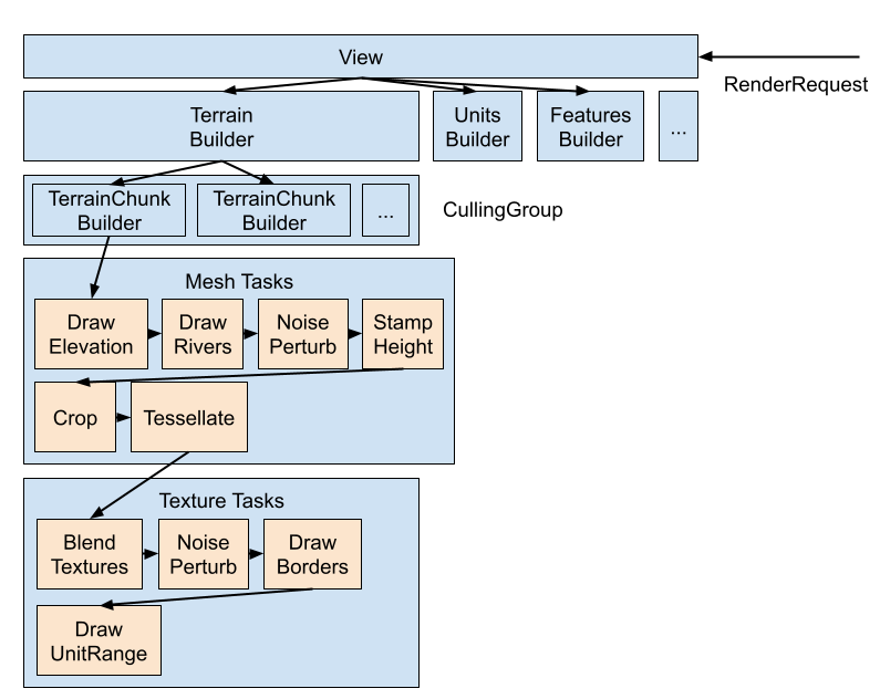
Note the sections in orange, which are the rendering stages running on the GPU (in compute shaders), which need to run in strict order since there are resource dependencies between them (texture and vertex data). However, as mentioned in the previous article, the RenderRequest system allows the ViewModel to only request the minimal necessary changes. As a result, these stages cache their intermediate results, so that the pipeline can be started somewhere in the middle if need be, and not all the way at the top. Alternatively, if only the borders need to be redrawn, the unit range doesn’t need to be redrawn, just re-overlaid.

Also note that as a result of the heightmap-based system, we can avoid re-rendering (cull) parts of the terrain that are offscreen since it is split into chunks. As such, each of the stages operate independently on a given chunk.

Stage Overview

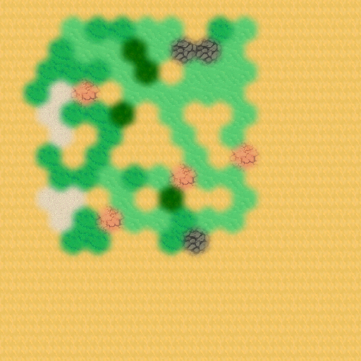
Below is a quick description of the stages shown above in the diagram. In this example, these stages are being used to render this final output:

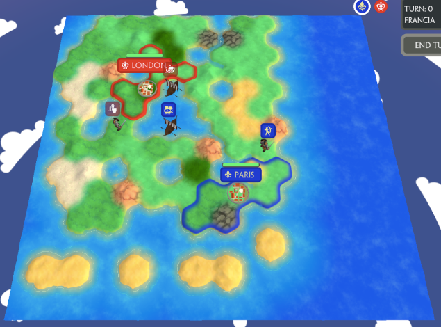
For simplicity’s sake, I’ve chosen a map that fits into just one chunk

Heightmap and Mesh Tasks

This first group of stages is responsible for creating the heightmap, and then the mesh from that.

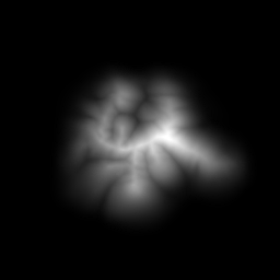
DrawElevation

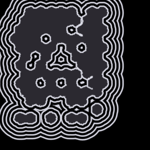
The input is a blank texture and the elevation data for each cell (above or under water). The output is a grayscale texture where elevation increases as intensity increases, like so:

DrawRivers

The input is the output from DrawElevation and the river data for each cell. The output is likewise, a grayscale heightmap, but with the riverbeds now drawn in, like so:

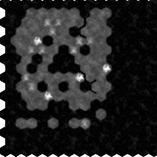
StampHeight

This stage places predefined terrain features like mountains onto the heightmap where applicable. The terrain features are created in a tool like GIMP to allow for quick and easy iteration:

Civilization 6. Windows PC, Firaxis, 2016.

and then added to the heightmap like so:

Note that one stamp is used for mountains, and another for hills. Also note that the overall intensity is scaled down to allow room for the mountains and hills to add more height.

NoisePerturb

This stage perturbs the results of the previous stage by:

1. Adding noise with a given scale, like: out[xy] = in[xy] + (scaleZ * noise.z)
2. Resampling data with a noise delta, like: out[xy] = in[xy + (scaleXY * noise.xy)]

The noise values come from a predefined coherent noise texture. This stage needs to fade noise down to 0 smoothly near the chunk edges so that chunk boundaries remain seamless. Below is the previous stage, but with noise applied:

This stage is later used after BlendTextures, but only with the second technique.

Tessellate

This final stage of mesh creation takes the heightmap generated so far and outputs a mesh object (the list of vertex data (position and UV) and triangle indices). As mentioned in part 1, this tessellation is a uniform square grid with configurable resolution.

One trick to reduce jagginess is to vary the diagonal chosen for a given square to line up with the underlying heightmap data.

Texture Tasks

After the mesh for each chunk is created, the texture to apply on each chunk is created as follows:

BlendTexture

This stage takes as inputs the cell biome data (e.g. tundra, tropical) and textures for each biome, and outputs a texture with the biome textures tiled and faded between each other like so:

Most of that sand will be underneath the water later

DrawBorders

This stage takes as inputs the output of the previous stage and the political borders of the map, and outputs a texture with these borders overlaid like so:

DrawUnitRange

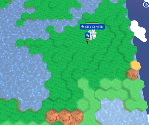
This stage takes as inputs the output of the previous stage and the movement or attack range of the selected unit, and outputs a texture with the range overlaid like so:

The unit north of Paris, south of the coastal mountain is selected

Smooth Cell Transitions

Approach 1: Blit and Blur

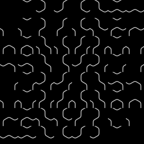
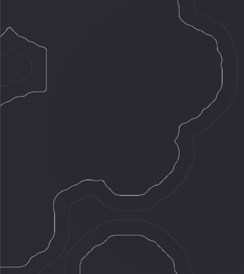
A naive implementation of the DrawElevation task would simply write a pixel value of 1 for a pixel that lies within an above water cell, and 0 for a below water one, like so:

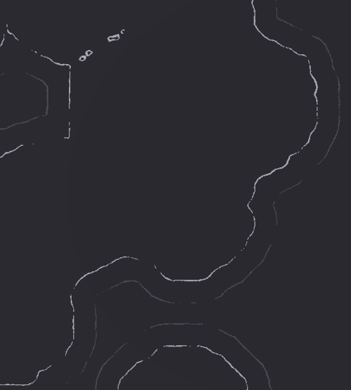
However, this results in a non-continuous heightmap where pixels just jump from 0 to 1. Worse, if we were to use the same technique for BlendTextures, it would become even more apparent:

One way to solve this would be to run something like a gaussian blur over this data. For BlendTextures, we can even use Texture Splatting so that we don’t blur the acual biome textures, just the biome texture boundaries. However, this breaks down at the boundaries of the chunk textures, since the blur won’t know what data exists in the adjacent chunks and will have to assume something, either clamping, repeating, or black, all of which are wrong and break chunk seamlessness when put together:

Padding?

To fix this, we could resize the chunk textures to be a little bit bigger than the chunks with some padding so that the blur has all the info it needs, and then crop them to size afterwards. I implemented this approach but was unsatisifed with it because:

1. Code complexity increased everywhere, as there are now 2 coordinate systems to deal with (padded vs unpadded)
2. Tweaking the blur radius requires tweaking padding to accomodate
3. Padding cuts a lot of the optimization from chunking, as the padded chunks now overlap and redo much of the same work

Finally, looking forward to drawing the rivers, the analogous approach would’ve been to:

1. Write 1s for pixels within a predefined distance from a river edge and 0 elsewhere
2. Blur this image for a smooth riverbed heightmap
3. Subtract this riverbed heightmap from the cell heightmap

However, this is almost certainly not the approach used in Civ, since Civ’s rivers look much more natural, as if they were designed by an artist, and not procedurally generated. The above approach would have smooth rivers, but all with straight bends at exactly 60 degrees.

Approach 2: Tileset

The approach I went with in the end was to essentially do the blurring offline, at asset creation time. The key insight was that instead of trying to blur the whole chunk of cells at runtime at once, once the elevations were known, I could instead define the transitions offline and then piece them together at runtime as needed.

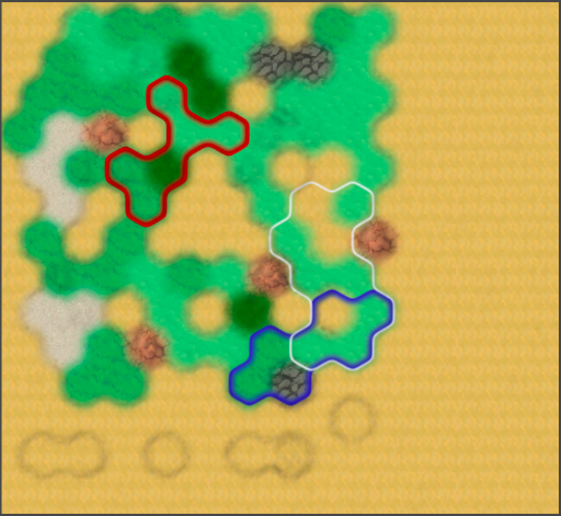
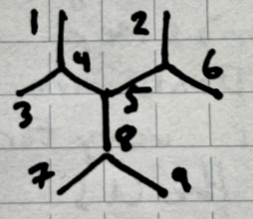
In a hexagon tessellation, there are 2 kinds of intersections:

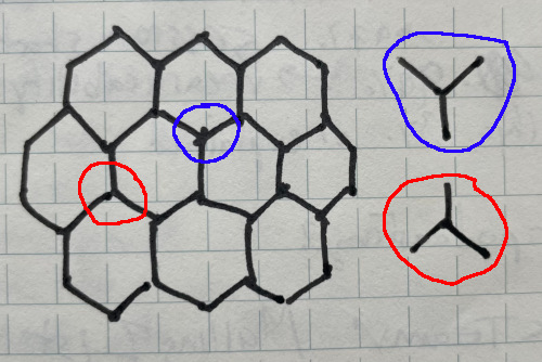
In red, “bottom” intersections, and in blue, “top” intersections

and these are just the same, simply mirrored about the horizontal axis, so let’s continue just describing the “top” intersections, the blue case. If I design a set of transitions to cover every possible case of elevation difference like this, then I can just tile these together at runtime and cover the entire chunk.

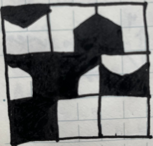
The tiles to use to compose a full map chunk

In this image, there are 8 tiles (the 9th is left over). Starting from top left, and going right and then down to the next row:

1. Is an intersection of 3 hexagons where the top (T) tile is below water, and the left (L) and right (R) tiles are above water.
2. T and L are above water, R is below water
3. T and R are above water, L is below water
4. L is above water, T and R are below water
5. R is above water, T and L are below water
6. T is above water, L and R are below water
7. T, L, and R are all below water
8. T, L, and R are all above water

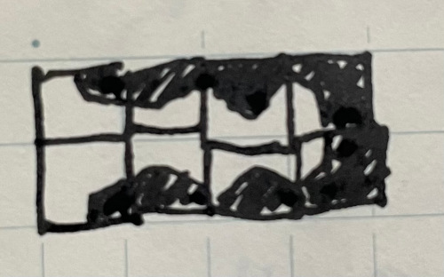
An example map chunk, composed from the above tiles (with some vertical flipping where needed)

With a little more precision and the blurring effect, the tileset can look like:

This solves the chunk boundary problem since every chunk is using the same strategy and tileset. This approach could still use some work because defining the transitions at the high frequency 3-hex level means that the output isn’t so natural. The artwork can mitigate this, but it’s still very apparent tiling is used, like in Civ 1:

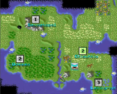
Civilization. Windows PC, MicroProse, 1991.

The artists do a great job making the tiles look natural, but it’s still very clear all the artwork is tile based. Notice how repetitive the river is.

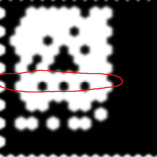
To mitigate this, one approach is to have a few artistic variations which stretch across multiple intersection tiles. This may be something I’ll come back to, but in the meantime, I simply made the scope of the intersections bigger, to cover not only the 3 hexagons involved in a given intersection, but also their 3 neighbor tiles, for a total of 6:

In this tile, L is above water and T and R are below water. In addition, the 3 outer hexagons, top left (TL), top right (TR), and bottom (B) are all above water as well.

With this scheme, it is possible to have more interesting patterns, as long as the tiles can be joined together seamlessly. The downside here is that there are more permutations: for a tileset describing every scenario – each one of the 6 cells can be either above or below water – this requires (2^6 = 64) tiles.

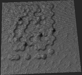
As a result, creating a seamless tileset that covers all cases from scratch is too burdensome. Instead, I generate the initial tileset with Python and ImageMagick (via Wand), which can then be edited by hand in GIMP for a more custom look. The gist of this tileset generation script is to, for every permutation: start with black, draw the above water hexagons in white, then blur each tile. Afterwards, the tiles are lumped together into one sheet. This is the final look of the generated heightmap tileset:

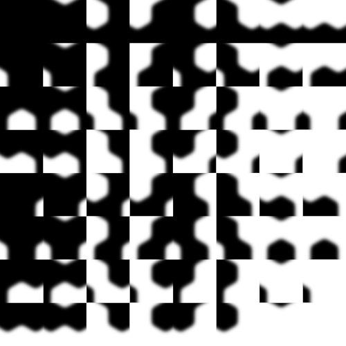
The 6-cell pattern is used for the heightmap blending but not for texture blending since the 3-cell pattern is not as noticeable behind all the biome textures. Since each of the 3 cells can be one of more than 3 different biomes, this leads to only (3^3 = 9) permutations.

Rivers

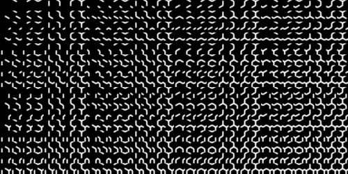
A similar approach is used to draw a tileset for the riverbed heights, recognizing that at each 6 cell intersection, there are 9 cell edges involved.

Each edge can either have a riverbed or not, so there are (2^9 = 512) permutations. This results in a tileset that looks like this:

Political Borders and Unit Range

Even though political borders and unit movement range boundaries are drawn on cell edges, they are really defined per cell, like cell height. For instance, a cell either belongs to Faction X or Faction Y (or none), and a cell is either within the unit’s movement range, or it’s not. As such, 2^9 permutations are not needed, only 2^6 are needed.

The tilesets for these thus resemble the height tileset:

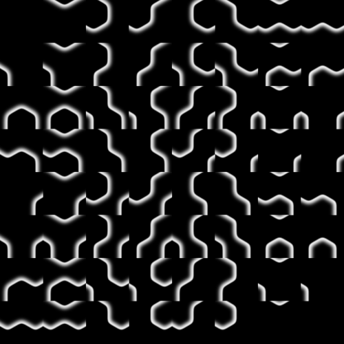
The political border tilesheet. Notice that the outside border edge is crisp, but into the interior of the owned cell, there is a gradient effect. The intensity is multiplied by the appropriate faction color at runtime.

The unit movement range tilesheet.

One important difference between drawing the heightmap and drawing the border and range effects is that the chunk’s texture is relatively low resolution. This is not noticeable for the biome texturing since the biome textures are interesting enough, but it is noticeable for border and range effects, since these are supposed to be sharp UI effects. So instead of drawing these onto the chunk textures directly, the border and range effects are instead drawn every frame in the chunk’s fragment shader.

To speed this up, the DrawBorders and DrawUnitRange tasks draw the following secondary textures, which are then used in the fragment shader:

1. BlendCoordsTex, a texture that in each pixel encodes the coordinates relative to the nearest 3-cell intersection point. The fragment shader then samples this to calculate interpolated UV coordinates, which it will later use for a given tile.
2. BorderTileMapTex, a texture array of N total channels (one per faction). Each channel contains a uint which is a bitset of which of the 6 cells the Nth faction owns. For each of the N factions, the fragment shader:
   1. Reads the bitset and picks the appropriate tile from the border tileset
   2. E.g., the value 000101 means the first (TL) and third (L) tiles belong to this faction, so the 5th tile in the tileset should be used.
   3. Samples the tile texture for an intensity
   4. Multiplies the sample by the faction color
   5. Adds the sample to the final pixel value, which may already include another faction’s color that is blending in or out
3. RangeTileMapTex, a 1-channel texture containing a uint which is a bitest of which the 6 cells are in the unit movement range. The fragment shader reads the bitset and picks the appropriate tile from the range tileset, then interpolating that tile texture, drawing it on top of the land texture

In this way, as much work as possible is offloaded to tasks that run infrequently (e.g. when a faction’s border changes from conquest, or the current unit moves) while still preserving crisp visuals.

Pipeline Architecture

In order to reason clearly about the stages, their intermediate outputs, and their dependencies, I adopted the following design:

class TerrainChunkBuilder {
  private ComputeShader shader;
  private DrawElevationTask drawElevation;
  private DrawRiversTask drawRivers;
  private RenderTextureSwap heightTex;

  public TerrainChunkBuilder(Rect chunkRect, CellRect chunkCellRect, ...) {
    drawElevation = new DrawElevationTask(chunkRect, chunkCellRect);
    drawRivers = new DrawRiversTask(chunkRect, chunkCellRect);
    heightTex = RenderTextureSwap.FromRect(chunkRect);
  }

  public void BuildLandMesh(RenderRequest request) {
    SetConstants(shader);

    drawElevation.Dispatch(request.Model, heightTex.Dst);
    heightTex.Swap();
    drawRivers.Dispatch(request.Model, heightTex.Src, heightTex.Dst);
    heightTex.Swap();
    ...
    landMesh = tessellateTask.Dispatch(meshSettings, heightTex.Src);
  }
}

Each task is defined in its own subclass of ComputeTask, which requires two things:

1. chunkRect, the dimensions of the chunk (to use for chunk texture size)
2. chunkCellRect, a hexagonal “rectangle” which describes which cells are contained within the chunk

As an example, DrawRiversTask looks like:

public class DrawRiversTask : ComputeTask {
  public void Dispatch(Model model, RenderTexture texSrc, RenderTexture texDst) {
    int kernel = shader.FindKernel("DrawRivers");
    ComputeBuffer cellRivers = CreateCellRiversBuffer(model.mapCells, chunkCellRect);
    shader.SetBuffer(kernel, "CellRivers", cellRivers);
    shader.SetTexture(kernel, "RiverTilesetTex", Assets.RiverTilesetTex);
    shader.SetTexture(kernel, "InputTex", texSrc);
    shader.SetTexture(kernel, "OutputTex", texDst);
    shader.Dispatch8x8(kernel, size);
  }
}

In general, a given stage draws “on top” of the results from the last stage, hence the texSrc and texDst parameters here. However, instead of creating N RenderTextures for each stage, we can instead just create 2 and swap between them until we’re finished. This is what RenderTextureSwap does, with Swap() just swapping what Src and Dst point to.

If we know there’s a certain point in the pipeline that will be started from frequently (unit range movement), then we can cache the result of the stage before that (biome texture drawing) in a texture, and start from there next time.

Water Effects

The water rendering makes use of a few effects:

1. The water becomes darker and more opaque the further it is from shore
2. Waves approach and break on the shore (zoom in :)
3. Caustic lighting

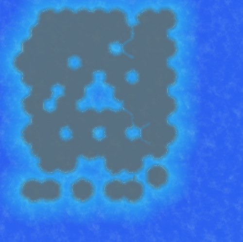
Distance Fields

In order to fade the water opacity and lightness, we need to know for each water pixel, how far it is from the shore. This can be done upfront with simple brute force, iterating over the entire heightmap and finding the closest above water pixel, to produce a distance field:

However, this is O(N^4) in the size of the texture, which is unideal. One technique I’ve learned about recently is jump flooding, which is much faster (O(N^2 log_2(N))). After using this technique, the one remaining problem is that this distance field cannot be calculated per-chunk independently, since we are excluding above water pixels that may be closer, but in a different chunk. As such, the algorithm has to run globally, across all chunks at once.

However, simply stitching all the chunk heightmaps together can result in a massive texture the GPU will refuse to work with. This is one reason why we split the map up into chunks in the first place! On the other hand, we don’t need pixel-perfect accuracy since this is being used for a fade effect. The solution here is to combine all the chunk heightmaps, but then bilinearly resize it to something small enough for the GPU to work with, and then create the distance field from that smaller image.

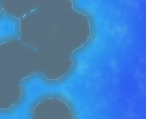
With the distance field in hand, it is then trivial to implement the first effect, by remapping the distance to the two colors and opacity.

Shore Waves

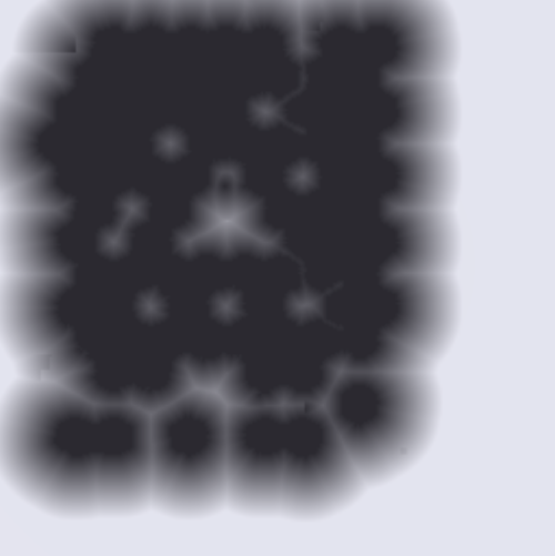
For the second effect, we can run a few functions over the distance field to create the waves:

1. First, run a sine wave over the distance field values. This creates a rippling from the shore:

Groovy, baby!

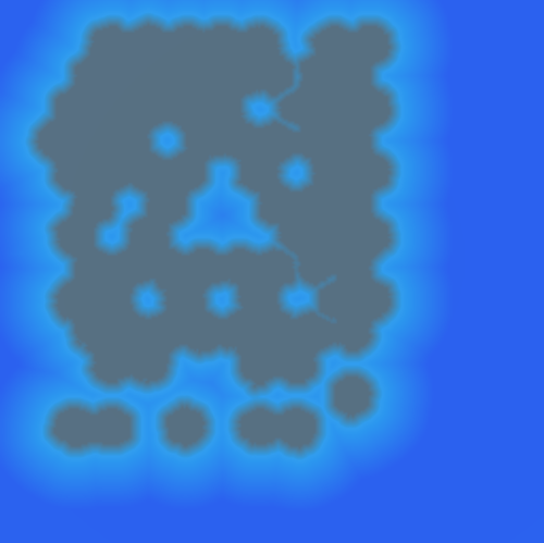
2. Cutoff pixels futher than a certain distance, since these should only be close to the shore. Fade the remaining pixels out by their distance to make further waves fainter.
3. Threshold the image by only taking values greater than say, 0.98. This means we only get thin bands, closer to wave crests.

4. Add noise to the inputs and outputs of the sine wave to make the result more natural looking, for the final effect. The noise also pushes pixels above or below the threshold, so it doesn’t look like one big unbroken wave, but (hopefully) like many small ones:

To make the waves approach the shore and break over time, simply add the current frame’s timestamp to the sine function.

Caustic Lighting

The caustic lighting is faked by playing with the noise texture as follows:

1. Sample the noise texture while scrolling through it by adding the frame timestamp to the UV coordinates.
2. Take the sine of this sample plus the frame timestamp (again) and the fragment’s world position.
3. Square this result and mask it with even more noise (The answer is always … more noise!)

The result from each of these 2 components (color/opacity + shore waves + caustic) can simply be added (assuming the weights are sane) for the final result (close up):

Future Work

I’m quite pleased with the architecture of the code, since it’s enabled me to try out radically different graphical approaches, like:

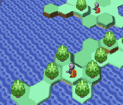
A GameBoy Advance visual style

A Nintendo DS pixelated style

A data model and style where cells can have finer grained elevation, beyond above/below water

Aside from gameplay, I’d be interested in taking a look at the following:

1. Lower level graphics implementation. In Unity, there is only so much exposed to the developer in order to maintain cross platform compatibility and to keep the API simple. I know newer underlying graphics APIs like Vulkan, Metal, and DX12 expose synchronization and resource dependencies explicitly, so it would be interesting to see how this task structure could be reimplemented upon those abstractions.

2. Spherical map. In most strategy games, the world is geometrically a cylinder, such that you can sail west and return from the east, but the poles are not a single point. Rendering on a sphere is more challenging since neither hexagons nor squares tessellate perfectly, so some workarounds include adding a few pentagons, or just making cell shapes more freeform.

3. Optimized mesh tessellation. In this implementation, the mesh is tessellated as a grid of uniformly sized squares. However, the seafloor for instance, is mostly flat and doesn’t need such detail, while conversely, mountain peaks are sharp and could use even finer detail. An interesting next step would be to implement a differential tessellation while still preserving seams between chunks so they can be culled as needed.